There are two standard modern imaging methods in (exploration) seismology: reverse-time migration (RTM) and full-waveform inversion (FWI). Both of these methods rest on the need for doing reverse-time wave simulations. The methods are often introduced with large amounts of mathematics, and complicated concepts such as “adjoints” and other such mathematical details. In my view, these complications are unnecessary for a first introduction to these imaging methods. In this blog post, I want to introduce RTM and FWI without any appeal to complicated math beyond a simple course in linear algebra and some vague knowledge of (partial) derivatives.

Reverse-time migration

Being an exploration geophysicist by training, I am quite familiar with the ideas underlying reverse-time migration. It’s a really rather simple method.

A simple modeling example

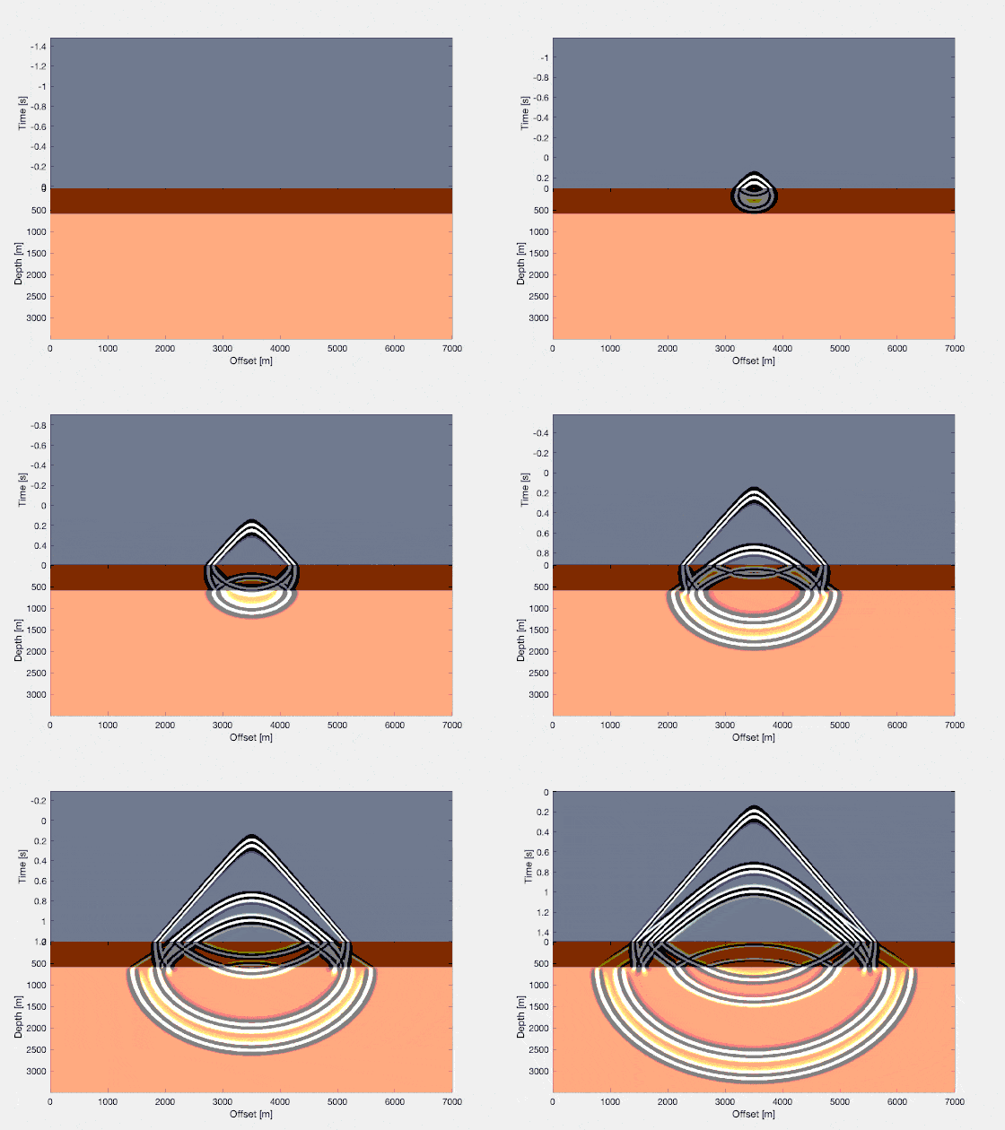
Consider a pressure wavefield in a simple model, where receivers are placed at (or close to) the surface. This shows you the idea of seismics in a simple way: waves propagate outwards from a source, and they interact with the different rock interfaces (in two different shades of brown). And in geophysics, we have access to the recordings of the wavefield over time. This is the image that you see at the top. It’s as if you’re dragging a piece of paper upwards while recording the properties of the wavefield at the surface (positive or negative pressure fluctuations, or particle displacements, or …).

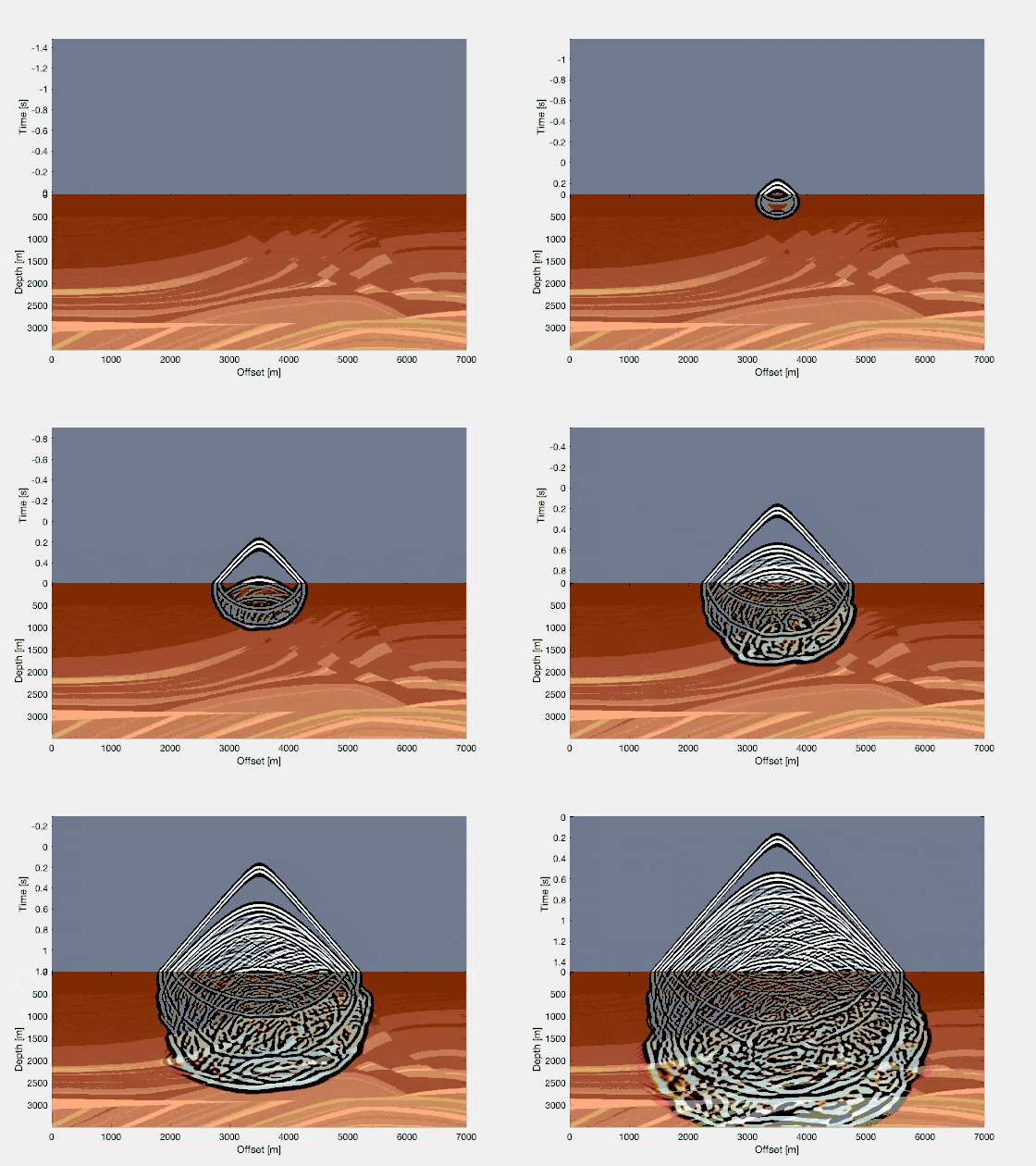
In reality, wavefields can be quite a bit more complicated. A famous model for seismic testing is the Marmousi model, and here we see a wavefield propagating inside the Marmousi model. Every shade of brown corresponds to a rock with slightly different properties in terms of the compressional wave velocity (i.e., how fast a wave propagates through that medium in units of “kilometers per hour”)! Again, in seismology you only have access to the wavefield over time, as measured at the recording states, thus: the gray part of the image on the top is all we have.

Splitting the wavefield into two parts

Now, we’re going to make a very obvious and very fundamental observation. We can say that, roughly speaking, a wavefield is composed of two parts: a source wavefield (which travels into the earth and is transmitted on each rock interface) and a receiver wavefield (which is generated at places where the source wavefield hits the interface between two rocks and which creates a reflection off those interfaces back up towards the surface). If you can get your hands on those two separate portions, then it is a simple observation to make that only at those locations where the source & reflected (or ‘receiver’) wavefield coincide in space and time, a rock interface was present. In the image below, each green line corresponds to a a wavefront at a given time. If you focus in particular on the (fictitious) event at 1 seconds, you see that the source and receiver wavefield only overlap at two points; the location of the rock interface.

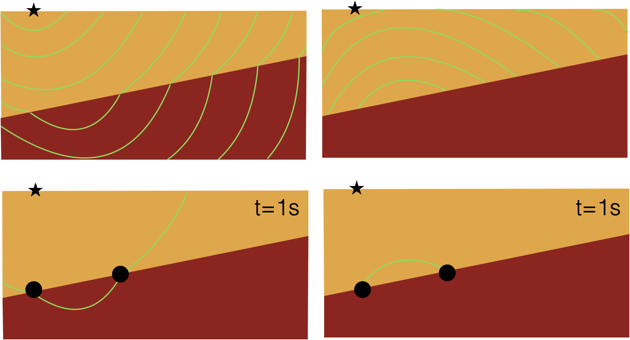
It’s a simple observation to make that, if you would point-wise multiply snapshots of the source and receiver wavefield for each time-step, you would only have non-zero entries at the location of the interfaces. This is what we will do for reverse time migration.

Creating the separated wavefields

How do you get those two wavefields separately, as we only have recorded data? Well, simply by modeling them in a smooth background model! Such a smooth background model may typically be available from other geophysical methods (such as traveltime tomography, full-waveform inversion, …). The use of a smooth model is absolutely essential, it means that as we model our source wavefield, it creates no additional reflections, and simply “purely” propagates into our domain.

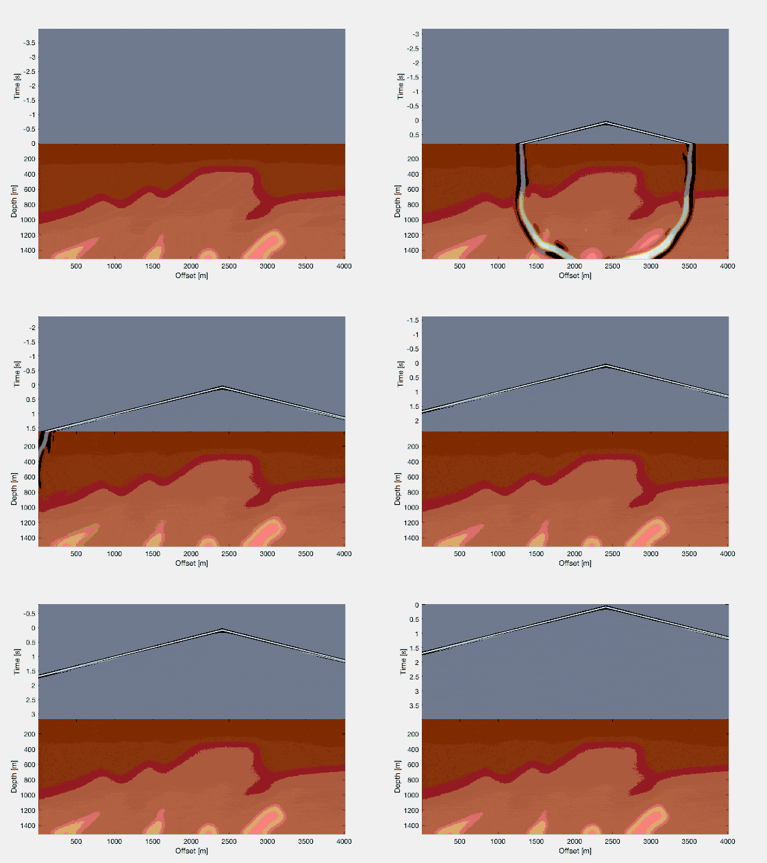
And then what about the reflected/receiver wavefield? Well, this one we model by using the actually recorded data in the following way: we model the wave equation in reverse time, and use our recordings as sources, in the way that we inject the recorded trace as a source into our model.

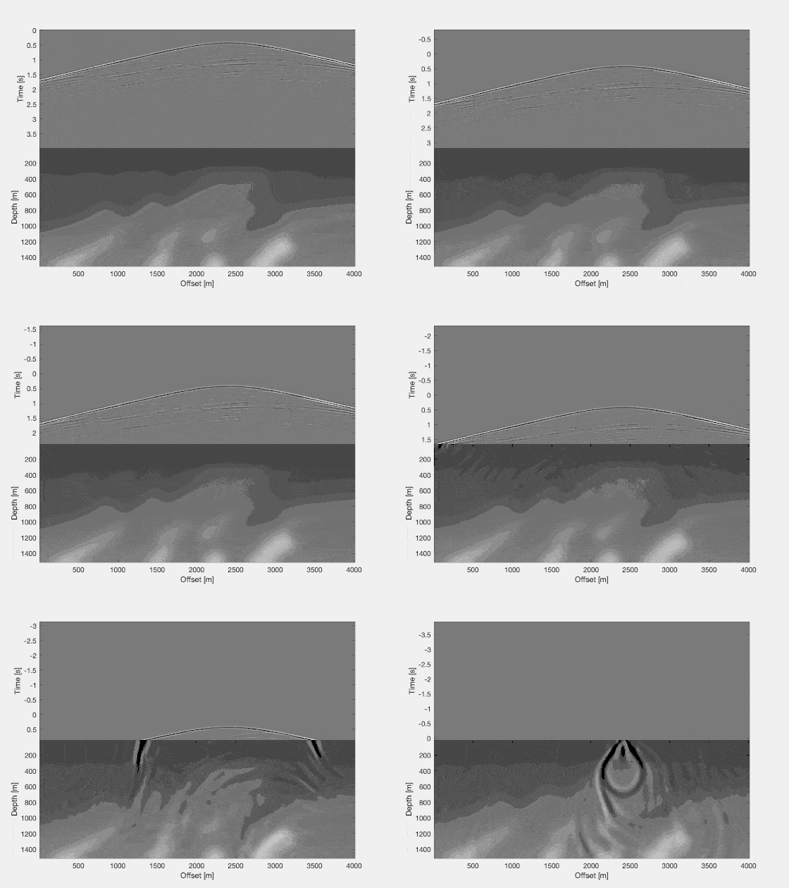
(this image is in gray-scale, such that you can still see the faint events on the recorded data, propagating into the model. I chose to make the gifs I use in these examples relatively small, so the quality isn’t great, but I want to keep the page loading time under control).

The creation of a reverse-time wave simulation is entirely straightforward, because the wave equation itself is fully time-reversible! Freely speaking, under zero initial conditions, that means that a solution satisfying the forward time wave equation also satisfies the reverse-time wave equation. All we have to do to create the reverse-time simulation, thus, is to appropriately inject our recorded wavefield as sources into the secondary simulation.

Time-reversing the source wavefield simulation

We require one additional step. Remember that I said that only where wavefields coincide in space and time, we have interfaces present? Well, right now, we have access to one wavefield simulation running in forward time, and another one running in reverse time. It’s hard to multiply snapshots at identical times. We do this either by storing all snapshots of the forward wave simulation in forward time (which can get quite expensive in terms of storage and I/O operations)…or by recomputing the wavefield in reverse-time. Similar to how we recompute the reflected wavefield in reverse-time, we can place virtual recording stations all around our model, and reconstruct the source wavefield in reverse time!

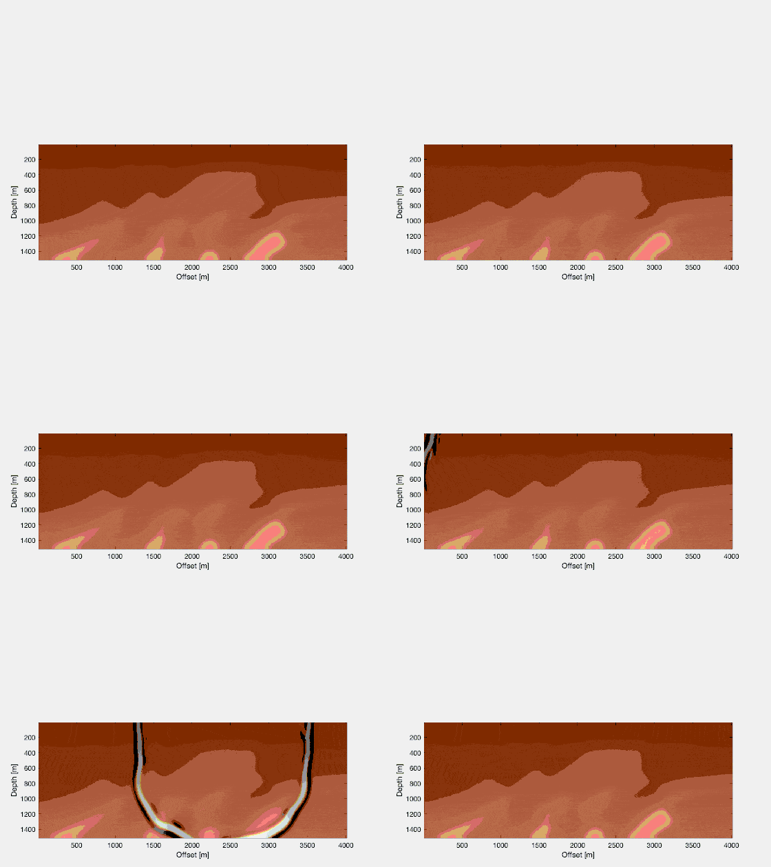
Creating the reverse time migrated image

Now, we have access to the source and receiver wavefield in reverse time. All we have to do, is to multiply each snapshot. In a language like MATLAB, we have a for-loop running from nt back to time 1, and we simply compute image = image + source .* reflected, assuming source and reflected correspond to the current snapshots of the two simulated wavefields. If we do that, we end up with a simple reverse time migrated image!

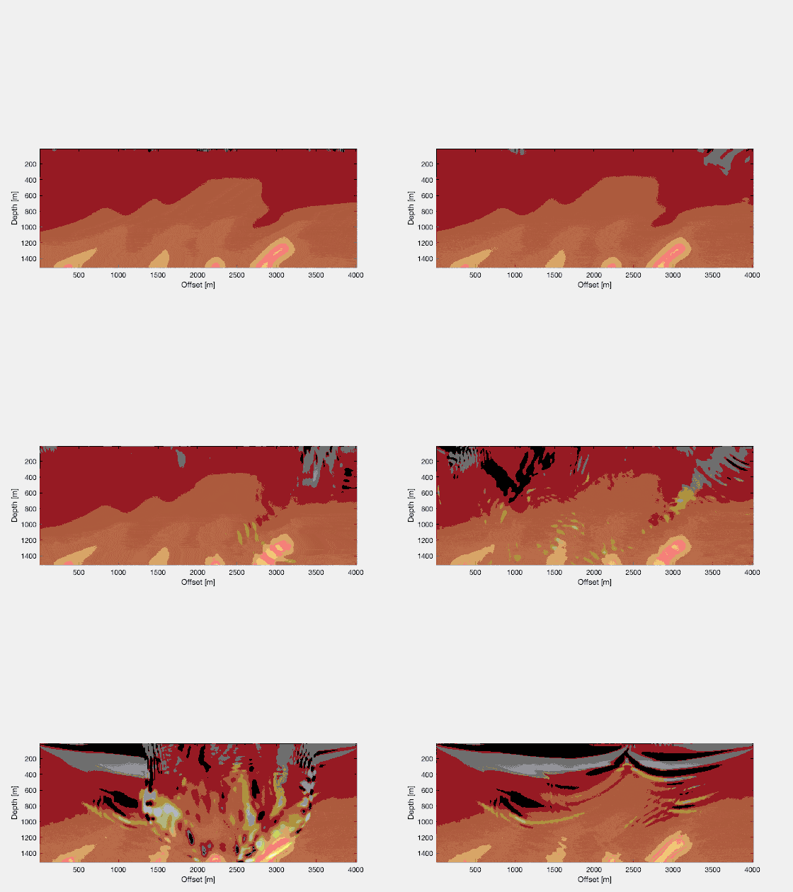
If you repeat this for a lot of shots, the noise will stack out, and you’ll be left with a good image. Other techniques are possible too, to further clean up the image. If you look at the final RTM image, for a large number of shots, you’ll see that it reflects the structural qualities of the original Marmousi model quite well! Just from running two wavefield simulations in parallel (and running three wavefield simulations in total), we can see a lot of details popping up! Quite a magical procedure.

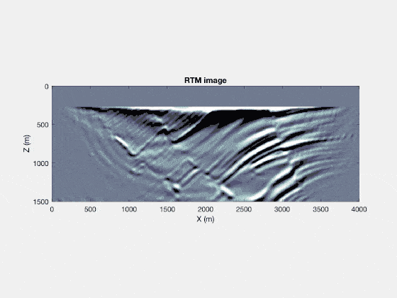
Full waveform inversion

In full waveform inversion (FWI), our goal is more ambitious. The idea is to find the velocity model that can explain our data. It turns out to work in a way that is extremely similar to a reverse time migration. A good way to get your hands on it, is by using the FWI lab from KAUST, which runs the following FWI example in MATLAB. It’s missing one file, which you must create after downloading the MATLAB files, which takes care of writing out the results to a binary short format.

function [] = write_bin(destination,seis)
fileID = fopen(destination,'w');
fwrite(fileID,seis,'float');
fclose(fileID);
end

The theory of full waveform inversion

The theory behind FWI is relatively complicated. Typically, the introductions take you pretty deep into the realms of Lagrangians, operator theory, Born approximations, and all that. I think that for a first introduction, this complexity is not actually needed, and we can get away with a LOT less mathematics. This is what I intend to do here in this blog post: de-mystify FWI for a first-time user.

A linear algebra trick

A large part of the efficiency of FWI is based on the following linear algebra ‘trick’, for vectors $\mathbf{y}$ and $\mathbf{x}$, and matrix $A$. We use a standard understanding of the inner product to find:

Notice, essentially, how we could move operator $A$ ‘through’ the inner product by taking the transpose of it. It has some pretty fundamental implications if you think about spaces and efficiency and all that, see the page on the Hermitian adjoint on Wikipedia. However, for our purposes, all that’s relevant is that this is an obvious linear algebra operation.

The cost function and discretized pressure field

Now, in FWI we want to minimize the difference between the observed pressure data at some receiver stations, $\mathbf{p}^\text{obs}(x_r)$ and our modeled version of that data, $\mathbf{p}^\text{synthetic}(x_r)$. The cost-function that we may write down for this problem is $ J = \frac{1}{2} || \mathbf{p}^\text{synthetic}(x_r) - \mathbf{p}^\text{obs}(x_r) ||_2^2 $, which is simply the ($L^2$-normed) difference between the synthetic and observed data. With some slight abuse of notation, we will consider it in particular as

to highlight the fact that the wavefields $\mathbf{p}$ are in principle existing for all $x$, we just single out those locations where there is a receiver, $x=x_r$.

Then, a note about what this discretized pressure field $\mathbf{p}$ really is, in my introduction to FWI. I’ve chosen for it to represent a vector with a rather strange hybrid identity. Any single element of the vector, $p_i$, corresponds to $p_i=p(x,i\Delta t)$. That is, any element $p_i$ corresponds to a full snapshot (for all $x$!), at a time $t=i\Delta t$. If we let $\Delta t \to 0$, this eventually starts to approximate a continuous signal, but this is not necessary for our purposes.

A model for the pressure field

The synthetic wavefield can, as the name suggests, be computed. It is thus fully deterministic. We assume that it solves the following wave equation,

for pressure $p$, the squared (!) wave velocity $v$, and a source located at $x=x_s$ with time signature $S(t)$. We will assume that $v$ is a constant, momentarily. However, the theory doesn’t really change for a non-constant velocity! A simple finite-difference approximation of the left-hand side gives

or an explicitly function to compute the solution at the next step is

For our discretized data-set, this corresponds to the following relation,

The gradient of the velocity model

Now we can start to make progress. What we’re really interested in is not the cost function $J$ itself, but how we can change the velocity model, in order to make the biggest changes in the cost function. In other words, we are interested in $\text{d}J/\text{d}v$. We can compute this with the chain rule,

We have used the properties of the inner product to write down the final expression. Now, the whole problem of FWI comes down to that term $\text{d}\mathbf{p}/\text{d} v$: how is the wavefield perturbed, if we make a perturbation in the (squared) velocity $v$? If we have a velocity model of 1000x1000 pixels, and we in principle allow all (1000x1000=)1 000 000 unique entries in our velocity model to vary (so this is the case of a non-constant velocity model $v$), then $\text{d}\mathbf{p}/\text{d} v$ asks us to compute how the wavefield gets perturbed for each individual perturbation of the velocity model. This would require 1 000 001 separate wavefield simulations, where we modify each of the individual parts of the velocity model, one by one, and compare them against the wavefield in the unperturbed state. That’s a lot of wave simulations!

Luckily, we can compute $\text{d}\mathbf{p}/\mathbf{d} v$ in another way, from a relation that we get from the wave equation itself. Namely, if we take the derivative of our relation $\mathbf{p} = \mathbf{F}(\mathbf{p}(v),v)$, we get

Okay, we can plug that into the inner product, and use the linear algebra trick!

Okay, it doesn’t look very nice perhaps, but we have actually achieved something very significant. The left-hand part of the inner product is fully independent of the velocity perturbations $\partial v$, and the right-hand side requires the derivative of the model equation to $v$, which is a trivial thing to compute!

Making the inner product more specific…

So, what is $\partial \mathbf{F}/\partial v$? Well, it is a vector $\Delta t^2\nabla^2 p_i$ for $i=[0,\dots,N-1]$. You can confirm this from simply looking at the properties of each individual $f_i$ as written above, and take the partial derivative to $v$. Not bad! And, then, what do we do on the “other” side of the inner product? Well, we’ll compute it in a particular way. Let’s say,

for

We can rewrite this relation a little bit by pre-multiplying the equation on both sides with the transpose term on the right-hand side, and then writing down a recursive identity for $\mathbf{r}$,

So, what is the exact form of $ (\partial \mathbf{F} / \partial \mathbf{p})^T$? Note that this is a matrix, $D_{ij}=\partial f_j / \partial p_i$ for $j=[0,N-1]$ and $i=[1,N]$. From the definition of the functions $f$, we see that this corresponds to:

This is thus a matrix with entries only on two diagonals.

If we use this property in the equation above, we find a remarkable thing,

We see, clearly, that for the final entry, $r_N = (p_N-p_N^\text{obs})\delta(x-x_r)$, and that for the other entries in the vector we have

Close inspection of the above relation shows that $r$ solves the finite-difference approximation of the wave equation in reverse-time, and we have to satisfy the property $r_N = p_N-p_N^\text{obs}$. The only way to compute that result is by, indeed, running the wave equation in reverse time, with as its source $(\mathbf{p}-\mathbf{p}^\text{obs})\delta(x-x_r)$, the misfit between the recorded and predicted pressure data, injected at the original receiver stations!

Oh, and by the way, the theory works equally well for a velocity model that is not constant in space. We would find the exact identical result.

An example of FWI

So, the recipe we’ve found is that to compute \(\frac{\text{d}J}{\text{d}v} = \left\langle r_{[1:N]}, \Delta t^2\nabla^2 p_{[0:N-1]} \right\rangle ,\) we require a scaled version of the pressure wavefield $\mathbf{p}$, and we require $\mathbf{r}$, which is the solution to the wave equation with as its source the misfit between the observed and predicted data. How does this relate to reverse time migration? Well, it’s very similar. We (1) compute a forward wavefield, in the current guess of the velocity model (not necessarily a smooth velocity model!), (2) we time-reverse the wavefield simulation of the previous step, just as with RTM, and (3) we compute a time-reversed wavefield with as its source the misfit between the obvserved and modeled data. Then we multiply the snapshots and sum all those results, just as with RTM. Indeed, we can show wavefields (2) as

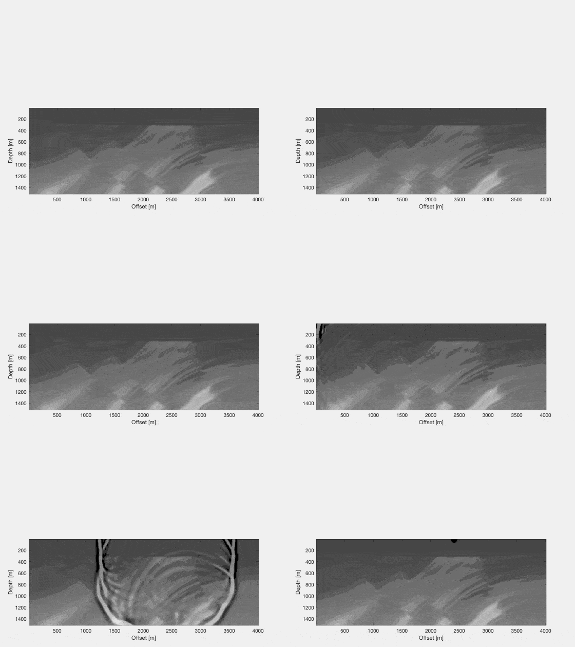
and wavefield (3) as

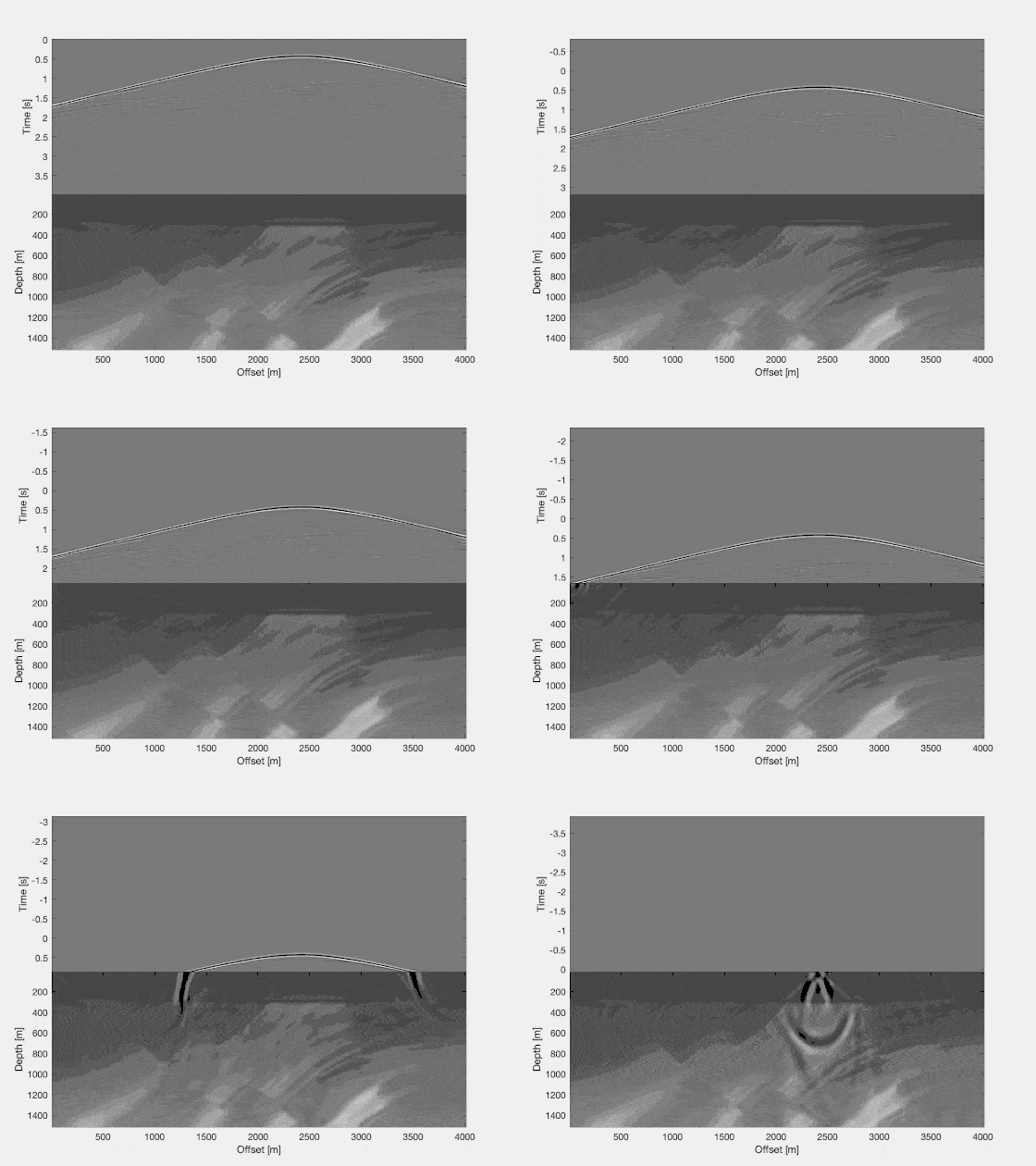
and the image computed is

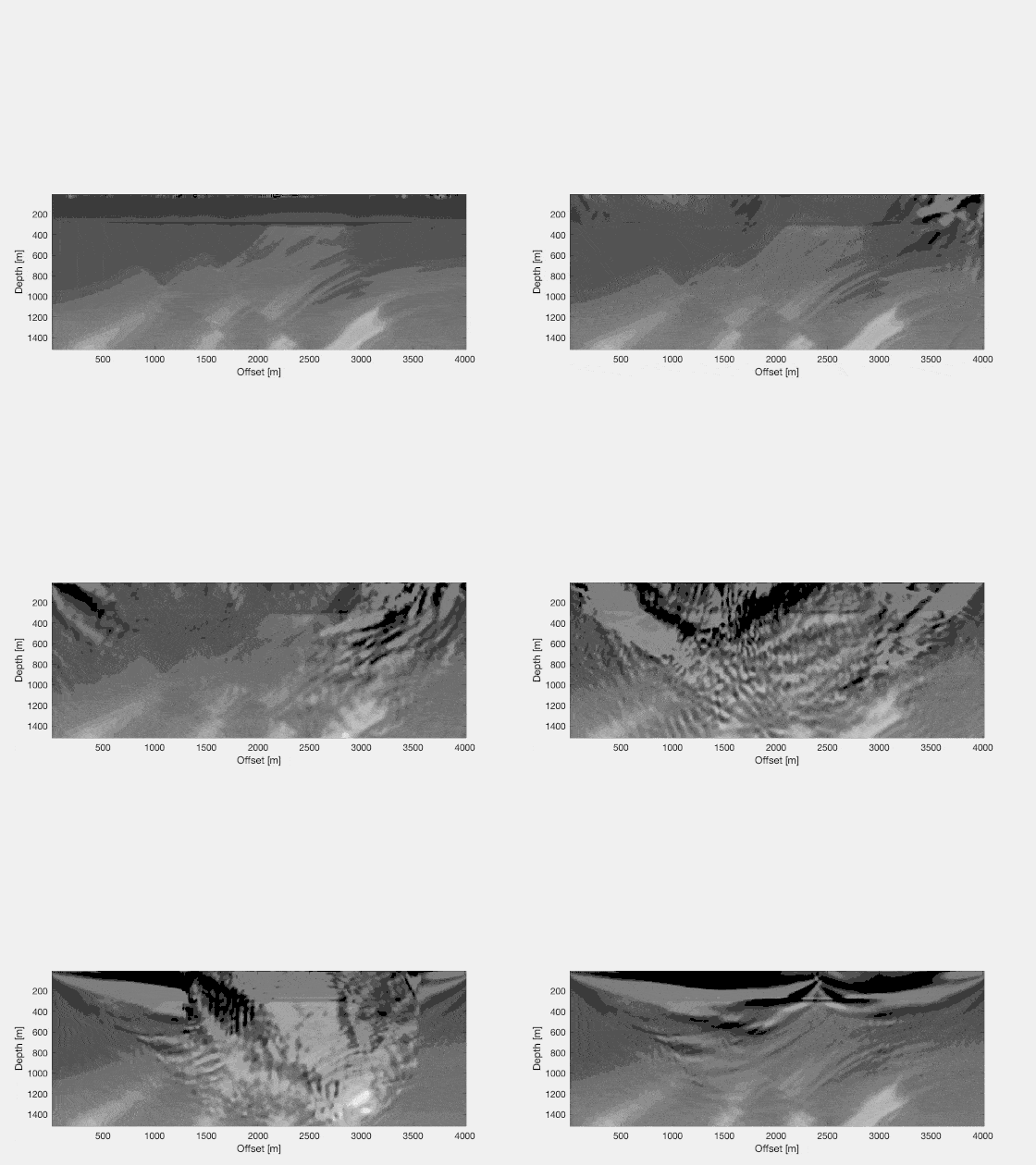
What this image tells us is how to update the model in order to decrease the cost-function. We would simply change our velocity model following the rule $v_{i+1}=v_i + \alpha \text{d}J/\text{d}v$, where we iterate through $v_i$ a number of times.

If you repeat this enough times, for appropriate step lengths $\alpha$, you (can) converge to the true velocity model. For example, you will find the following result

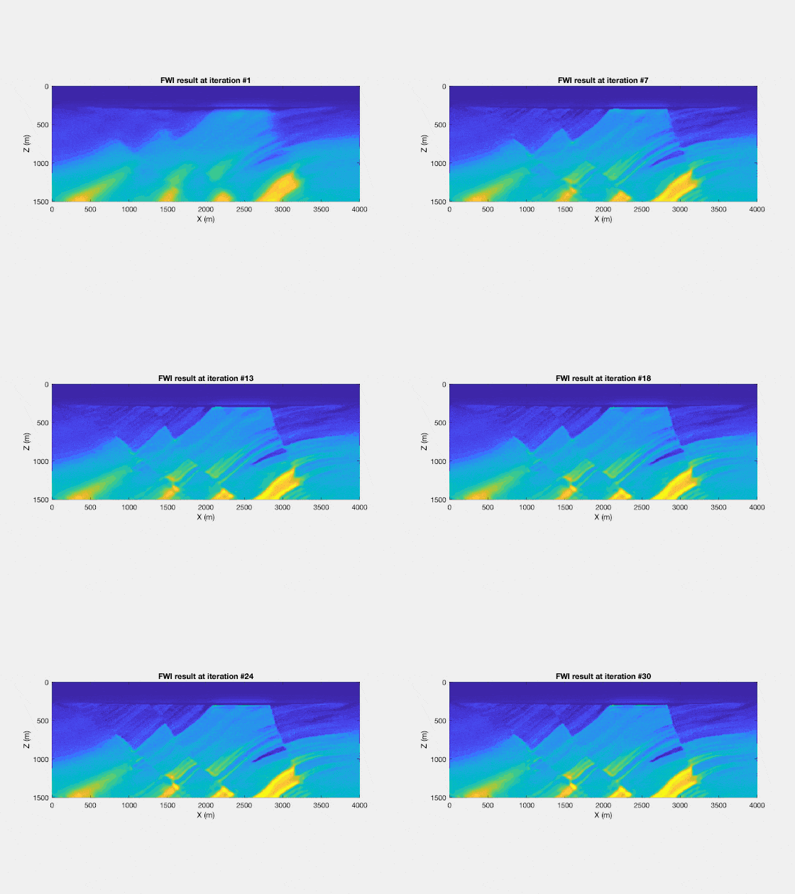
And with that, I finish my introduction to a computation of full waveform inversion, without all the complicated math of Laplacian multipliers, operators, working in the frequency domain or with use of other assumptions. Of course, those other more complicated methods have their merit, as they allow us to generalize FWI in a strict and rigorous way, including the theory for (much) more complicated wave physics and much more complicated models (with anisotropy, density variations, …). But, for a first introduction, I think that the theory as described here is a lot simpler, as it doesn’t require any mathematics beyond some simple linear algebra.