Time dispersion corrections
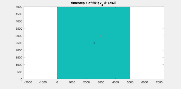
In the modeling of seismic waves, we typically integrate over time using a finite-difference approximation. When we use small steps in time, these approximations are more-or-less correct, but these simulations can be computationally intensive. When we use a large time-step for these finite-difference approximations, the simulation is cheaper but can also contain seeming errors, as shown on the gif below.
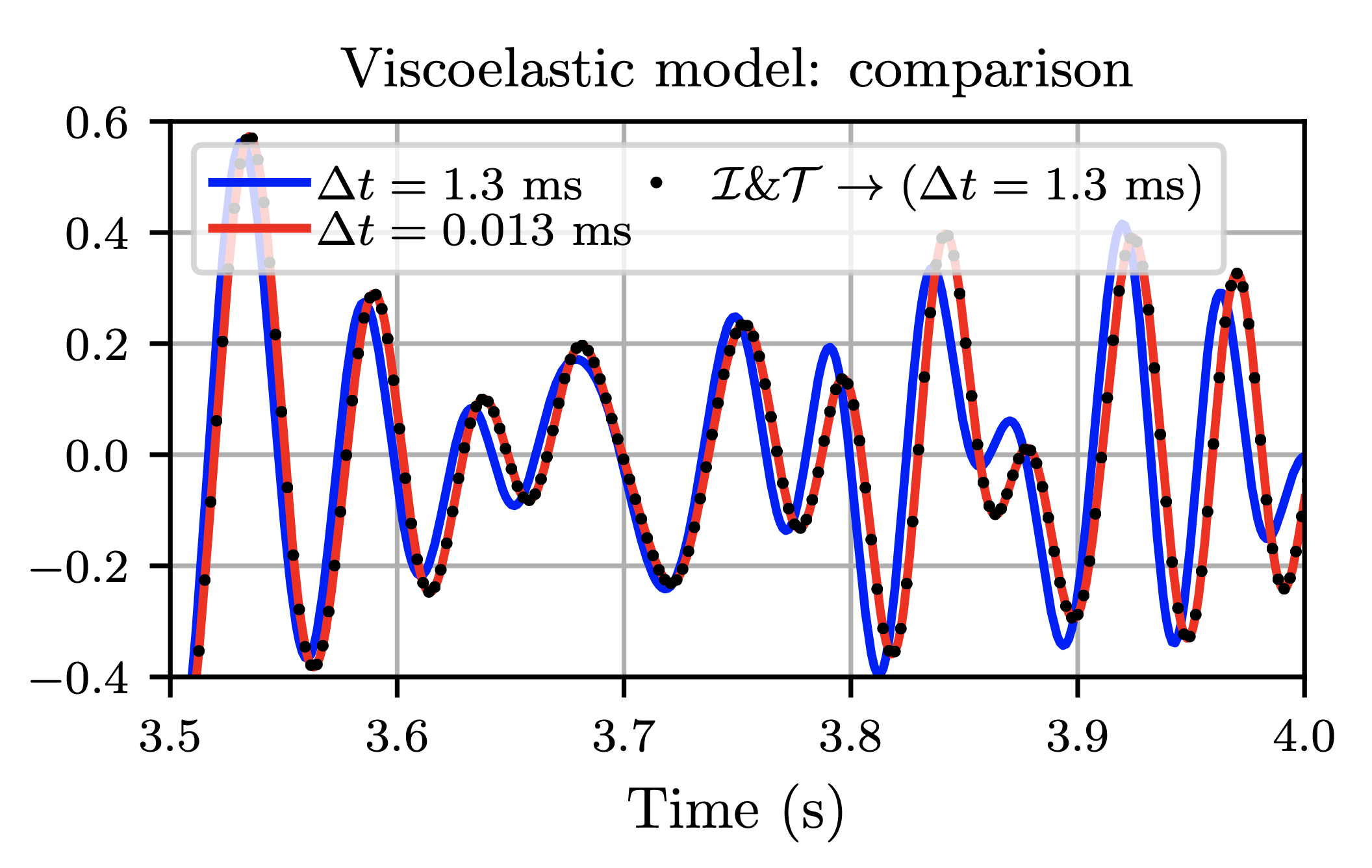
We have explored a way to use the large time-step for the finite-difference approximations (i.e., compute results in a cheap way) and filter out the errors using a pre- and post-propgation filter of negligible cost. We have shown that this even holds for viscoelastic wave simulations. For example, on the figure below you see in red a computationally expensive simulation (2+ hours) with a small step in time. In blue you see a computationally cheap simulation (80 seconds) using large steps in time – but the blue solution is clearly erroneous when compared to the red solution. The dotted solutions uses the filters for the cheap simulation (coming out to 80.1 seconds, 0.1 seconds extra for the pre- and post-propagation filters), and overlaps with the correct solution excellently. Hence, we can obtain accurate results at a very low cost.
Optimal finite-difference coefficients using the Remez exchange algorithm
I have studied the design of “optimal” finite-difference coefficients. Those coefficients have a minimal error, while spanning a large frequency/wavenumber range. That means that the optimal effect of the finite-difference coefficients produce the following error plot:
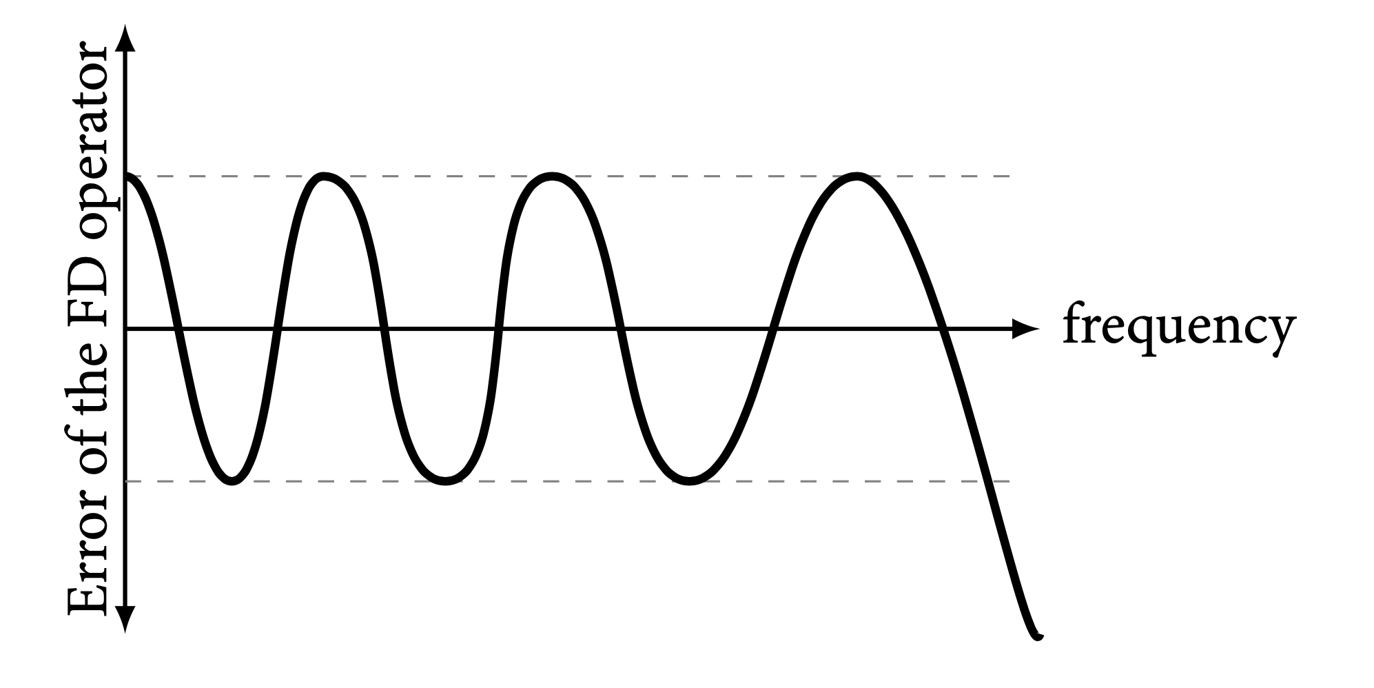
I managed to generate such coefficients rapidly (within a second) using the Remez exchange algorithm, a know technique from the digital signal processing field. It works in a simple way. We initialize a (random) guess for the optimal coefficients and look at the extrema in the error plot. We change the coefficients such that the extrema are assigned to some error level. In this process, new extrema will be formed. This is iterated until we reach the desired optimal set of coefficients.
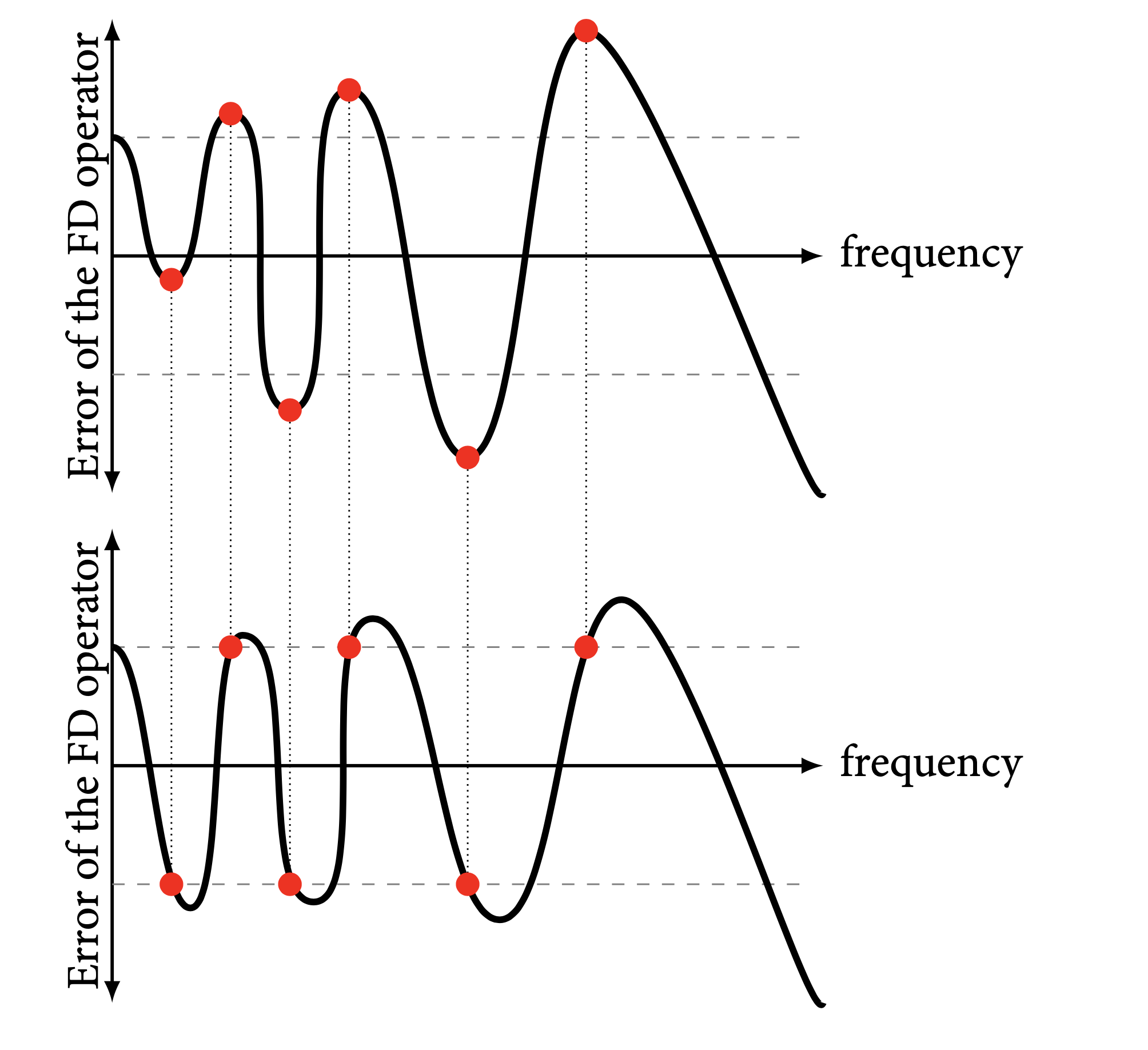
The effect of these optimal coefficients is that we can simulate high-frequency waves with only limited error levels – much smaller error levels than traditional finite-difference methods. More-over, I generalized the entire theory to apply to arbitrary finite-difference operators, using samples from arbitrary offsets, and applying to three separate cost-functions. In passing, the theory also makes it straightforward to compute a quick “least-squares-optimal” operator.
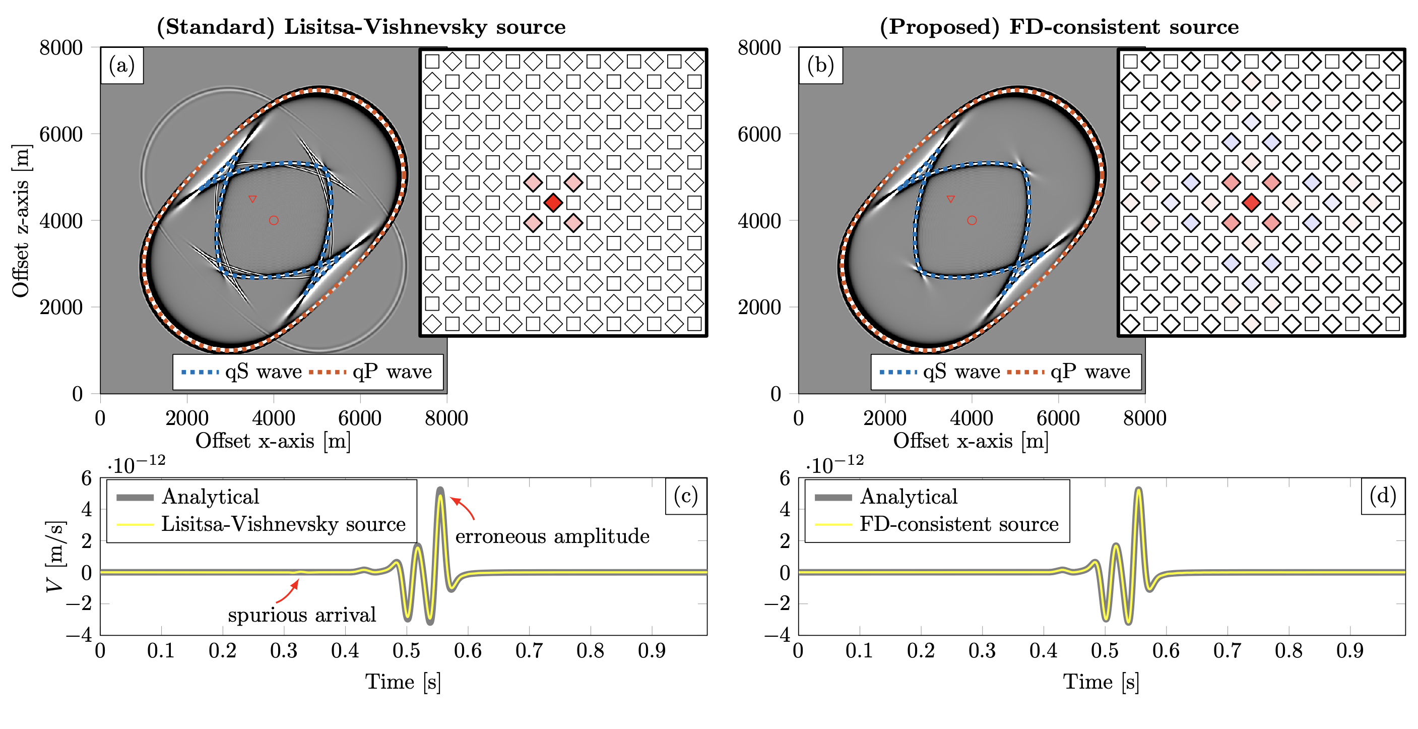
The FD-consistent point-source
I developed a new formulation for the introduction of sources on finite-difference grids. The standard introduction of point-sources makes an intuitive appeal to correctness, but gives wrong results. For example, in this anisotropic medium, a standard point-source results in

while the FD-consistent point-source that I worked on results in
The response computed with the FD-consistent point-source is correct, while the standard source is not. For example, this is shown with the following figure, showing that our proposed method computes an accurate response with respect to an analytical solution, while the standard alternative does not.